Learn
Trading Cost Sensitivity: How Much Cost Can a Strategy Survive?
At a glance
Cost sensitivity asks how a result changes when trading costs change, and at what cost its average reaches zero (the break-even cost). In our frozen sample of 23,899 fair value gap (FVG) retest events, the historical mean reached zero at about 7.7% of the assumed cost allowances (0.077× baseline): mean gross expectancy was +0.020R, while the original assumed costs averaged 0.260R per event. At the full allowance the mean was −0.240R. This is a cost repricing of unchanged fills, not a broker quote, execution simulation or forecast.
On this page

A backtest can look profitable because its assumed cost is small. The useful next question is how much room remains before that result reaches zero—and whether the average hides trades whose cost is much larger than their planned price risk.
We ran a new secondary analysis on 1 October 2026, using the completed fair value gap (FVG) retest events from our original study. We kept the entry rules, exits and 12 datasets unchanged. This article explains the calculation, the distribution behind it and what an execution test still needs to establish.
Freeze the trades before changing the cost
There are two different experiments:
Scroll horizontally if needed
| Experiment | What changes | What it can answer |
|---|---|---|
| Reprice a frozen event list | The cost deducted from each existing result | How much of the observed result remains under that cost assumption? |
| Rerun execution under different conditions | Bid/ask prices, fills, delays, rejected orders or other execution behavior | Which trades would occur, and at what prices, under that model? |
Our analysis does the first. Increasing a cost allowance does not change whether a limit order fills or a stop triggers. It does not reproduce a wider spread’s effect on entries. TradingView also distinguishes simulated slippage from the problem of unfilled limit orders; its broker emulator uses explicit fill assumptions. TradingView strategy documentation.
The source sample contains 23,899 completed events of the FVG retest model (model A in the original study), with the original minimum gap of 0.25 ATR. Concurrent events are allowed. R is each event’s gap width in price units; it is not 1% of an account and does not describe a portfolio return. Read the original FVG methodology for the entry/exit rules and histories.
Calculate cost in the same units as the result
For each event in this particular model:
cost_R = round_trip_price_cost / gap_width
net_R(m) = gross_R − m × cost_R
m is a multiplier. At 0×, the calculation deducts nothing. At 1×, it deducts the original allowance; at 2×, twice that allowance. Each instrument retains its own baseline cost:
Scroll horizontally if needed
| Market in the original study | Baseline round-trip allowance | Unit |
|---|---|---|
| NQ continuous futures | 0.50 | Index price points |
| ES continuous futures | 0.35 | Index price points |
| EURUSD | 0.00012 | Quoted price units, equivalent to 1.2 pips using a 0.0001 pip |
| XAUUSD | 0.35 | Quoted price units |
These are the study’s fixed combined assumptions, not current broker quotes, minimum achievable costs or observed execution charges. The analysis scales the whole allowance. It cannot identify how much of a difference comes from commission, spread or slippage individually.
A hypothetical example shows why the denominator matters. A 0.10 price-unit allowance divided by a 1.00-unit gap costs 0.10R. The same allowance divided by a 0.20-unit gap costs 0.50R. Equal price costs need not mean equal R costs.
For a result in account currency, use currency-denominated costs at the matching trade size. For a return in basis points, normalize costs to the same notional. Do not subtract pips, dollars and R directly from each other.
The same events at eight cost levels
Every row below contains the same 23,899 completed events, weighted equally per event rather than equally per market. We recomputed each event’s net result, positive-outcome status and profit factor at each level. The multiplier scales all four market-specific allowances together; it is not a universal spread setting.
Scroll horizontally if needed
| Cost multiplier | Mean net result | Positive outcomes | Profit factor |
|---|---|---|---|
| 0× | +0.0201R | 33.80% | 1.030 |
| 0.10× | −0.0059R | 33.80% | 0.991 |
| 0.25× | −0.0450R | 33.80% | 0.936 |
| 0.50× | −0.1101R | 33.78% | 0.853 |
| 1× | −0.2403R | 33.34% | 0.714 |
| 1.50× | −0.3706R | 32.66% | 0.605 |
| 2× | −0.5008R | 31.98% | 0.518 |
| 3× | −0.7613R | 30.49% | 0.392 |
A positive outcome means net R strictly greater than zero. Profit factor here divides the sum of positive net R by the absolute sum of negative net R. Neither number is an account-level performance statistic.
Notice the first two rows: the positive-outcome percentage is unchanged to two decimals while the mean crosses zero. Costs can reduce winners and deepen losers without immediately changing which events remain positive. A win-rate headline can miss that deterioration.
Find the break-even cost multiplier
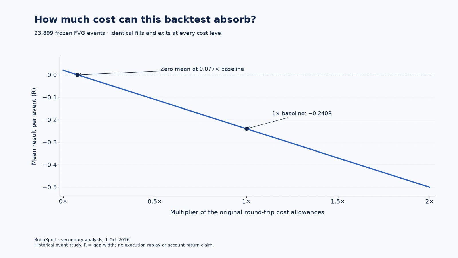
Because the fills stay fixed, the mean is linear in the cost multiplier, so the zero-mean (break-even) multiplier follows directly:
mean_net_R(m) = mean_gross_R − m × mean_baseline_cost_R
zero_mean_multiplier = mean_gross_R / mean_baseline_cost_R
Our unrounded means are approximately 0.020122R gross and 0.260460R cost. Their ratio is 0.077257, or about 7.7% of baseline. At that multiplier the historical mean is zero; above it the mean is negative under this model.
This does not mean that reducing a broker’s spread by 92.3% would produce a deployable strategy. The baseline is an assumed combined allowance, the pooled result mixes markets, and repricing does not change fills. It is a descriptive threshold for this sample. When the gross mean is already negative, no nonnegative cost can make it reach zero by subtraction alone.
Why median cost gives the wrong expectancy
The pooled cost distribution at 1× baseline is uneven:
Scroll horizontally if needed
| Cost statistic | R per event |
|---|---|
| 10th percentile | 0.017R |
| Median | 0.100R |
| Mean | 0.260R |
| 90th percentile | 0.700R |
| 99th percentile | 2.400R |
We use empirical nearest-rank percentiles: sort the costs and take observation ceil(p × n). For even-sized samples this can differ from averaging the two middle values, or from the original engine’s upper-middle median convention.
Subtracting the median cost would suggest 0.020 − 0.100 = −0.080R. The actual mean after costs is about −0.240R. To calculate mean expectancy, subtract mean event-level cost, not median cost and not cost divided by average gap width.
A separate two-event hand check makes that last point visible. Suppose both events pay one price unit but their gap widths are 1 and 4. Their R costs are 1 and 0.25: an average of 0.625R. Dividing one by the average width, 2.5, gives 0.4R, which is wrong for the mean of those two normalized costs. This check is included in the downloadable code.
All twelve datasets, including the exceptions
The following thresholds use each dataset’s own cost allowance and historical events. Different timeframes cover different date ranges; this is not a controlled ranking of instruments.
Scroll horizontally if needed
| Dataset | Completed events | Gross mean | Net mean at 1× | Zero-mean multiplier |
|---|---|---|---|---|
| NQ M5 | 2,030 | −0.0191R | −0.0636R | None: gross negative |
| NQ M15 | 1,877 | +0.0502R | +0.0215R | 1.750× |
| NQ H1 | 1,834 | +0.0913R | +0.0735R | 5.132× |
| ES M5 | 2,073 | +0.0131R | −0.2124R | 0.058× |
| ES M15 | 1,859 | +0.0287R | −0.0836R | 0.256× |
| ES H1 | 1,815 | +0.0109R | −0.0514R | 0.175× |
| EURUSD M5 | 2,534 | −0.0556R | −1.2599R | None: gross negative |
| EURUSD M15 | 2,115 | +0.0575R | −0.4627R | 0.110× |
| EURUSD H1 | 1,853 | +0.0484R | −0.1652R | 0.227× |
| XAUUSD M5 | 2,168 | +0.0321R | −0.1391R | 0.188× |
| XAUUSD M15 | 1,851 | +0.0402R | −0.0398R | 0.502× |
| XAUUSD H1 | 1,890 | −0.0302R | −0.1315R | None: gross negative |
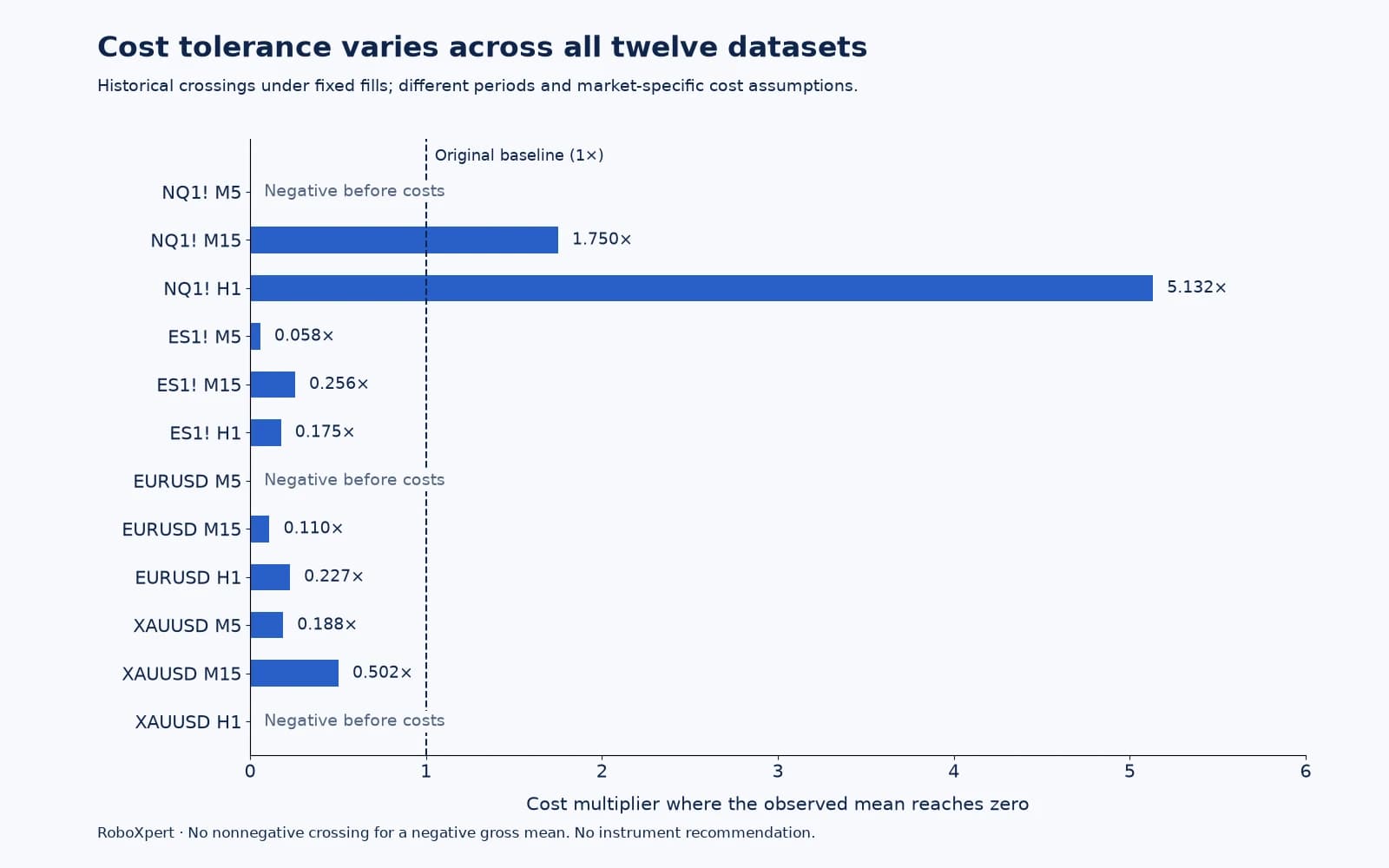
NQ M15 illustrates a time-period caveat. Its full-sample crossing is 1.750×, but the original earlier-period subset gives 2.128× and the later subset 0.652×. Thus a positive whole-period result at baseline hides a negative later-period mean at that cost. NQ H1 remains positive at baseline in both subsets, but it is also the best of twelve observed cells; that selection is not a new validation sample.
The original 70/30 boundary is based on fill time. Trades crossing the boundary were not purged. We call this a historical stability comparison, not a clean prospective out-of-sample test.
Does removing expensive events solve the problem?
We grouped every completed event by its cost in R at baseline, without changing the strategy. These are descriptive groups chosen for analysis, not independently validated filters:
Scroll horizontally if needed
| Baseline cost group | Events | Gross mean | Mean cost | Net mean |
|---|---|---|---|---|
| 0–0.10R | 12,118 | +0.0299R | 0.0438R | −0.0139R |
| Above 0.10–0.25R | 5,716 | +0.0246R | 0.1622R | −0.1376R |
| Above 0.25–0.50R | 2,861 | −0.0028R | 0.3581R | −0.3609R |
| Above 0.50R | 3,204 | −0.0043R | 1.1679R | −1.1722R |
Even the lowest-cost group has a negative mean after the assumed costs. That finding does not rule out every alternative filter. It does show that “just remove the most expensive events” is not a demonstrated repair here. Any changed entry rule needs a separate, documented test rather than replacing this baseline after inspecting the outcome.
Apply a cost test to your own backtest
Start by identifying which costs are already in the input result. If your reported P/L already includes commissions or bid/ask execution, subtracting those again will double count them. In TradingView, commission settings can be percentage-based, per contract or per order; commission applies at entry and exit. Its slippage setting uses ticks and affects market and stop orders. Record the actual properties used. Official strategy properties.
The same check applies to an Expert Advisor tested in MT5. The Strategy Tester can configure commissions, and its profit calculation in pips omits commission and swap calculations, so a report is only interpretable alongside its configuration. MetaTrader’s testing documentation.
Then make the analysis reviewable:
- Freeze the source run. Save the rules, version, history, fill model and original cost settings. Retain event count and file hashes.
- Choose one accounting unit. Distinguish entry-side charges, exit-side charges and whole round-trip amounts. Explain how volume and partial exits are handled.
- Vary stated assumptions. Label zero, baseline and stress scenarios. An arbitrary 2× allowance is a stress assumption, not proof of realistic execution.
- Inspect the distribution. Show mean, percentiles, thin winners and the relevant market/time breakdown. Keep unfavorable cells visible.
- Separate repricing from execution. If spread changes fills or exits, run an execution-aware test as a separate experiment. Limit-order queueing and failed fills cannot be repaired by a fixed deduction.
- Compare with observed demo or live records when available. Match the symbol, size, session and order type; keep demo and live evidence distinct.
The companion backtest versus live guide explains why matching a historical curve is not enough.
Reproduce the calculation and respect its limits
The kit contains the new standard-library Python analysis, the unchanged original engine, sanitized input manifest, aggregate results, source/data hashes and methodology notes. Synthetic arithmetic checks run without market data. An exact historical rerun requires the original permitted TradingView exports; raw market data is not redistributed.
We verified all twelve input hashes, recreated the original completed FVG retest event counts and matched the original rounded gross and baseline net means. Additional checks cover heterogeneous gap widths, zero and negative gross means, monotonic cost curves and complete cost-bucket accounting.
The same limitations as the original study remain: overlapping events; unequal histories ending 29 September 2026; 1-, 3- and 15-minute intrabars; unresolved continuous-futures back adjustment; unfinished-event exclusion; possible final-bar incompleteness; and no account capital, financing or margin model. This secondary analysis adds cost scenarios, not independent market evidence or statistical significance.
Reader resource · ZIP
Inspect and reproduce the cost analysis
Python analysis, original engine, aggregate results, method notes and input hashes. Synthetic checks need no market data; rerunning the historical events requires the original permitted exports, which are not included.
Download the cost-sensitivity kit
Sources & further reading
Your next question